implicit 4D grapher

View the project here: https://4dgrapher.netlify.app/

Introduction

Objects live in $\mathbb{R}^4$ (the fourth dimension) with coordinates $(x,y,z,w)$.

Humans can only perceive a 3D perspective projection of this space, so our goal is to project 4D points down into something viewable on our screens.

We’ll use a one point projection along the $w$ axis, meaning all objects seem to get smaller as they get further away, converging towards a single “vanishing point” on the horizon line. The visible 3D space is one “slice” of the full 4D object.

1. Projection

Projection lets us take higher-dimensional points and turn them into lower-dimensional ones. For example, 3D-appearing objects on your screen, like in video games, are often actually 3D points projected onto your 2D screen.

Let’s recall the 3D case. With an eye/camera at $(0,0,d)$, screen at $z=0$ and point at $(x,y,z)$, the new projected point is at:

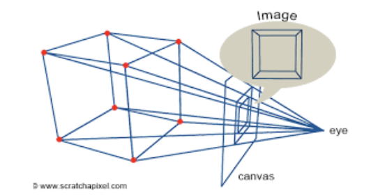
The key idea is that points farther from the camera are scaled down. This formula is derived through similar triangles, pictured above.

We can then extend this idea directly to $4D$. Projecting along $w$ (as we defined), the scale factor becomes:

Our projected coordinates are:

This gives us a 3D point from a 4D one that we can actually render.

2. Rotations

Since we’re working in 4D, we need to use rotations to gather more information about our 4D object.

If a 2D object rotates around a point and a 3D object rotates around an axis (or a line), then a 4D object must rotate around a plane.

First — how many rotations are there in a 4D space? Planes are defined by 2 axes, and there are 4 axes total — meaning there are $4$ choose $2 = 6$ possible rotations. These are $xy, xz, xw, yz, yw, zw$.

We can split these into two groups: a) Rotations entirely within 3D space: $xy, xz, yz$ b) Rotations involving the fourth dimension: $xw, yw, zw$.

A rotation only affects the coordinates of the plane it operates in. For example, an $xw$ rotation changes only the $x$ and $w$ coordinates of a point.

To see where the formulas come from, start with 2D. If we have point $(a,b)$, we can write this in polar form:

If we rotate by $\theta$, the new angle becomes $\epsilon + \theta$ but the length is preserved:

We can then use the angle addition formulas for $\sin$ and $\cos$:

And now we plug in our original assignments for $a$ and $b$ to get:

We can plug in any values to check that this makes sense!

This generalizes cleanly to higher dimensions. For an $xw$ rotation in 4D, for example:

The other rotation planes follow the same pattern.

3. Updates

After coding my basic projection and rotation functions up, it’s time to focus on the actual rendering!

Day 1

Before anything I quickly coded up a rotating cube in 2D, just so I can make sure all my projection math is correct. This works! YAYYYY!!!

Day 2

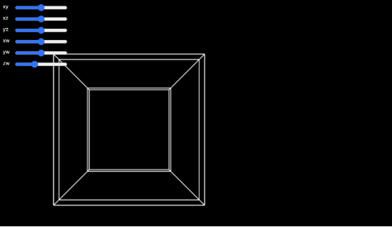
First, I tried to render a tesseract to test the full pipeline from 4D → 3D → 2D. I defined a hypercube’s points and edges manually. The final algorithm was pretty simple: I wrote a draw loop that updated the rotations based on slider inputs every frame. Seeing it move correctly was very satisfying.

Day 3

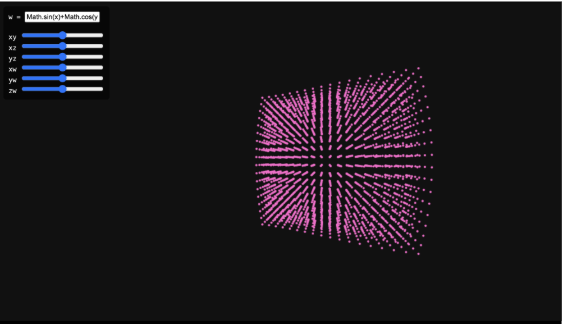
I added a textbox so the user could input any function! For now, functions had to be inputted in JS syntax (like math.cos()) and didn’t support anything super fancy. I wasn’t sure how to graph this continuously in 4D space, so I sampled random points, plugged them into the inputted function, and then graphed and displayed them. This led to a collection of points that sort-of resembled the function — if you squinted your eyes a little bit.

Day 4

I was busy at school today, but I quickly coded a “mesh” that would connect neighboring points with lines and give the illusion of more continuity. This did not work. At all. Points only connected within the same $x$ value, producing a distorted mess…

Day 5

After a little bit more research, I’m going to try and rewrite my code almost entirely using three.js. I also considered writing my own graphics engine, but using existing tools will let me focus more on usability. This was supposed to take a day. (spoiler: it did not).

4. How WebGL Works

Modern 3D rendering is built on triangles. In order to graph a triangle, you need three non-collinear points and then edges to connect them. This process of rendering vertex data into pixels is known as a graphics pipeline. This turns out to be a rather complicated process, and WebGL handles much of this. Since my project isn’t super low-level, I’m using three.js, a high-level library built on top of WebGL that makes the entire rendering process a lot easier.

We begin by setting up a standard three.js scene, with a scene, perspective camera, and a WebGLRenderer. The perspective camera is super important, which mirrors the same idea as our projection math earlier. Three.js handles this a lot more efficiently than I first implemented via a projection matrix.

User navigation is handled using OrbitControls, which implements a damped orbital camera model. This allows rotation around the origin while keeping the camera at a fixed radius, making it easier to inspect the geometry of the 4D shape without changing anything about the camera transforms manually.

5. Back to Updates

Day 5 con’t

I attempted to triangulate neighboring vertices directly. After hours of debugging, I realized that I was trying to render around 1.5 million triangles (connecting every single set of neighboring vertices!!), which was far more than my GPU could handle.

Day 6

I wanted something working with three.js, so for now, I just reverted back to my original points. It looks a lot better, I can render more points without it crashing and it looks pretty cohesive. I’m happy I got something to work.

Day 7: learning the marching cubes algorithm

To solve the triangle explosion problem, I’m going to use an algorithm called the marching cubes algorithm.

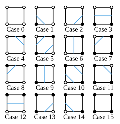
Here’s a high level explanation: let’s use “marching squares” as an example, which is the same algorithm in 2D. First, we label a sample of points as being either “inside” or “outside” the function (whether it satisfies some condition of the function). Then, we draw a grid, and each square is stored in something called a voxel. For each “square” in that grid, we split them up into 16 cases, simplifying it to a different output per combination of points. Then, if we want, we can use linear interpolation to “smooth” out the points. The 3D version works exactly the same way, except we have 256 total configurations instead of 16.

More formally, marching cubes extracts an implicit surface from a scalar field, mapping $f:\mathbb{R}^3 \to \mathbb{R}$. This means that every point in 3D space gets assigned a single number.

Real world examples include: temperature in a room at a specific point, density in a fluid, or in our case, the value of $f(x,y,z,w)$.

An implicit surface is defined by choosing an isovalue $c$ and taking all points where $f(x,y,z)=c$. Since we want to render a 3D space instead of 4D, we set $w$ as a constant (referring to the specific “slice” of the function) and apply the projections/rotations to $(x,y,z)$.

A scalar field samples space on a regular 3D grid and assigns a scalar to each coordinate. We store one scalar per grid point, so $\text{field}[i][j][k] = f(x_i, y_j, z_k)$. For efficiency, we flatten this to a 1D array using index $i \cdot n_y \cdot n_z + j \cdot n_z + k$.

A voxel (cube) is defined by 8 neighboring scalar-field samples. Each corner is classified as “inside” or “outside” the surface based on whether its scalar value is above or below the chosen isovalue. We encode this into an 8-bit index:

where $b_n$ is 0 or 1 based on the corner’s classification. This gives us 256 possible cases.

For edges flagged in the edge table, we find the exact intersection point using linear interpolation:

This is what allows the surface to appear smooth rather than aligned to the grid. After computing all intersection points for a voxel, we connect them to form our surface!

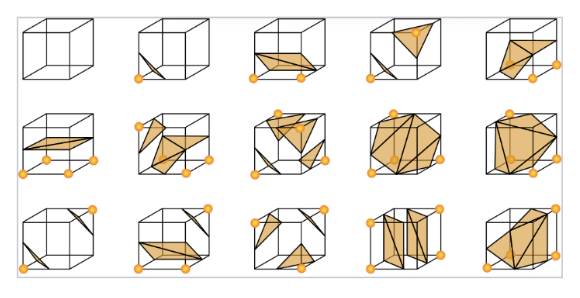
A second lookup table, the triangle table, specifies how to connect the interpolated edge points into triangles for each of the 256 cases. These triangles are added to a global triangle list. Once all voxels are processed, the result is a triangle mesh approximating the implicit surface!

Day 8: implementing marching cubes

After learning the marching cubes algorithm, I wrote an implementation in Python without relying on any outside libraries. This was super inefficient and could only render a few triangles at a time — the triangles would also fade in and out of view when rotated.

Day 9: Switch!

I finally came up with a slightly different algorithmic pipeline, which solved all of my problems!

Some of the key changes: instead of implementing the marching cubes algorithm from scratch, I used three.js’ built-in marching cubes function, which simplified the process and was more computationally efficient.

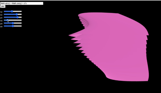
The new, improved (and finished!!!) algorithmic pipeline: define $f(x,y,z,w)$; choose a specific $w$ value as a “slice” controlled by a slider; rotate the coordinates using user input; generate a 3D grid for $(x,y,z)$ and evaluate the function at each point; run marching cubes to output a triangle mesh; display with three.js.

Changing $w$ or any of the rotation angles triggers the algorithm to run again and recompute the 3D surface. This allows interactive visualization of the 4D function.

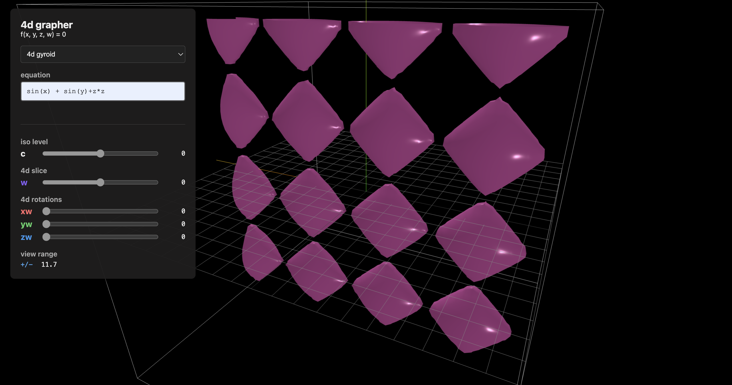
I now have a working 4D grapher!

Day 10: Cleaning up UI

I finalized the UI: making it prettier, adding a 3D viewer in the shape of a box around the function (this was a lot harder than I expected).

Conclusions

There are a lot of flaws with this project — the sliders are often janky (due to collisions with .getElement), half of the graph disappears when you zoom in (I still don’t know what causes this), and there are a lot of things I could add to make this project more polished. However, for a ten-day project, I’m really happy with how it turned out! Check out the code on my github page: (coming soon!)